FIG. 31How It Works
Map projections: why Greenland looks as big as Africa
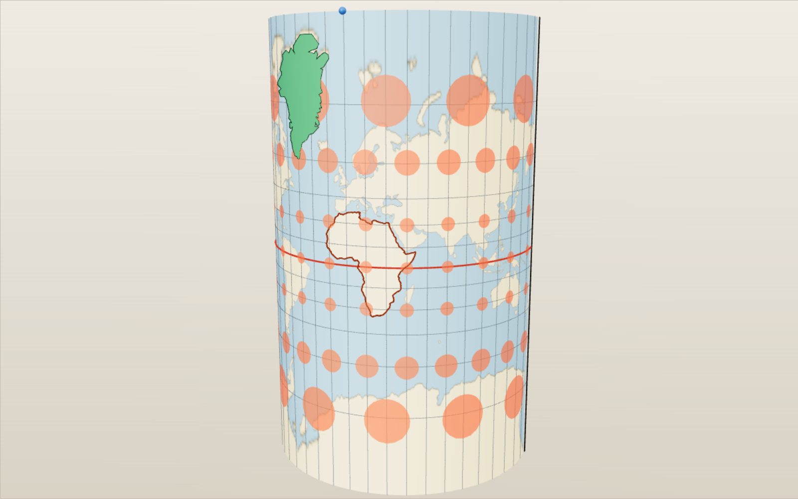
On a Mercator map Greenland looks bigger than Africa, which is in fact about 14 times larger.
This device cannot show the 3D model. You can read the guide steps below as text.
1 / 20 On the globe every circle is the sameThe red circles are all 500 km in radius, from the equator to 75° N. Nothing is stretched yet. Drag to turn. Scroll or pinch to zoom.
Drag to turn. Scroll or pinch to zoom.
What the model shows
Greenland looks as big as Africa on a Mercator map because that projection enlarges areas far from the equator. A flat map cannot preserve every property of a globe at once. Comparing projections shows which ones preserve areas and which preserve angles.
Look at a classroom world map and Greenland seems about as big as Africa. On a globe it is a modest island next to a huge continent. Neither picture is wrong on purpose. A sphere cannot be pressed flat without stretching some parts of it, and every flat map chooses where the stretching goes. This exhibit shows that choice being made, one point at a time, for 25 different maps.
The model starts as a globe of radius 1. The slider marked "Globe to map" wraps the globe in paper, cuts the paper and lays it flat. What the paper is depends on the projection. For Mercator and its relatives it is a cylinder touching the equator. For the transverse Mercator it is a cylinder lying on its side, touching one meridian. For the conic maps it is a cone over the middle latitudes, which opens into a fan. For the azimuthal maps it is a flat sheet touching the globe at one point, and for three of them (gnomonic, stereographic and the satellite view) a small lamp shows where the light comes from that throws the shadow. The last map puts the globe on an icosahedron and unfolds its 20 faces. Press play and the model repeats the move, globe to map and back.
The globe is covered by a grid of 144 by 72 cells (72 by 36 on slow phones). Each corner of the grid is placed by the formula of the chosen projection, and the coastline picture rides on the grid, so the continents stretch exactly as the formula says. The red dots are Tissot circles, each 500 km in radius. The green shape is a country you can drag anywhere; it starts as Greenland, and the lab under the controls offers 34 others. The brown outline is Africa, which stays put as a yardstick. The purple and orange lines are two routes between two cities: the shortest one and the one that keeps a single compass heading. The panel in the corner keeps score: the projection, what it keeps true, the area scale at the country's centre, how big the country comes out on the map and how many times it fits into Africa.
Under the controls there is more. The projection list explains all 25 maps and marks what each keeps true. The size table shows the country you picked on every projection at once, sorted from smallest to largest. The route tool gives distances and headings. Tap the flat map and the model measures the distortion at that point. Six tasks ask you to find a particular map, and 48 cases set up famous maps, uses and size comparisons with one press.
Why a globe will not lie flat
Try to flatten half an orange peel and it tears. The peel is curved in two directions at once, and paper is not. You can roll paper into a cylinder or a cone without stretching it, because those shapes are curved in one direction only. A sphere is different: its curvature is the same in every direction at every point.
Carl Friedrich Gauss proved in 1827 that this curvature is something a surface keeps no matter how you bend it, as long as you do not stretch it. A flat sheet has zero curvature and a sphere does not, so no amount of bending turns one into the other. Every flat map of the world must stretch some distances and shrink others.
What a map can do is choose what to protect. It can keep angles correct in every small neighbourhood, so that a tiny circle on the globe stays a circle on the map; such maps are called conformal. It can keep areas correct, so that every country takes up its fair share of paper; those are equal-area maps. It can keep distances true along certain lines, or from one point. It can make every great circle a straight line. But it cannot do all of these at once, and in particular no map is both conformal and equal-area. The badges in the projection list show which choice each map makes.
How a globe becomes a flat map
Most projections are not real shadows. They are formulas that take a latitude φ and longitude λ and return a point x, y on the paper. Still, the old picture of wrapping paper around the globe helps, because it tells you where a map is accurate: wherever the paper touches the globe, the map has true scale.
A cylinder wrapped round the equator touches it along the equator. Unroll it and you get a rectangle where meridians are straight vertical lines, evenly spaced, and parallels are straight horizontal lines. All cylindrical maps share that grid. They differ only in how far apart they put the parallels. Spacing them by ln tan(45° + φ/2) gives Mercator. Spacing them evenly gives the plate carrée. Spacing them by sin φ gives Lambert's equal-area map.
A cone set over the globe like a lampshade touches it along one parallel, or cuts through it along two. Unrolled, it becomes a fan: meridians are straight lines meeting at the apex and parallels are circular arcs. Conic maps fit countries that stretch east to west in the middle latitudes, like the United States, China or Europe.
A flat sheet touching the globe at one point gives an azimuthal map. Directions from that centre point are true on all of them. Here three are real perspective projections. With the lamp at the centre of the globe you get the gnomonic map. With the lamp at the point opposite the centre you get the stereographic. With the lamp infinitely far away you get the orthographic, and with the lamp at a satellite's height you get the vertical perspective. The azimuthal equidistant and the Lambert azimuthal equal-area use the same sheet but place each point by a formula rather than by light.
Some maps fit none of these. Pseudocylindrical maps such as the sinusoidal, Mollweide, Robinson and Equal Earth keep straight parallels but bend the meridians inwards towards the poles. The Goode homolosine cuts the map open in the oceans. The icosahedron map wraps the globe in 20 triangles and unfolds them. The model uses the cylinder animation for the pseudocylindrical maps too, so you can watch the meridians bend as the paper unrolls.
Mercator keeps angles and gives up sizes
Mercator wanted a chart on which a ship's course of constant compass heading, a rhumb line, is a straight line. Then a navigator can lay a ruler between two ports, read the angle against any meridian and steer that angle.
On a cylindrical map the meridians are parallel, while on the globe they meet at the poles. At latitude φ the real distance between two meridians is only cos φ of what it is at the equator, yet on the map it stays the same. So every parallel is stretched east to west by 1 / cos φ, the secant of φ. To keep small shapes undistorted, Mercator stretches north to south by exactly the same factor. The spacing of the parallels is the sum of all those little stretches, and works out to y = R ln tan(45° + φ/2).
You can check the numbers in the model. The 60° parallel lands 1.317 Earth radii above the equator, and the 75° parallel 2.028 radii. At 85° it is already 3.131 radii up, and the parallel there is drawn 11.47 times longer than it really is. The pole itself would be infinitely far away, so the map stops at 85°.
Because both directions are stretched by sec φ, areas are stretched by sec² φ. At 30° that is 1.33, at Seoul's latitude of 37.57° it is 1.59, at 60° it is exactly 4 and at 75° it is 14.9. In the model the red Tissot circles stay round, which is what conformal means, but the circle at 60° is twice as wide as the one at the equator and covers four times the area.
Web Mercator and the transverse Mercator
The map on your phone is almost Mercator. Web maps cut the world at 85.0511° north and south, the latitude where the map becomes exactly as tall as it is wide. A square world can be split into 4 square tiles, each of those into 4 more, and so on for every zoom level. Google's documentation describes this tiling, and the projection is registered as EPSG:3857, "Pseudo-Mercator". The "pseudo" is there because web maps take latitudes measured on the slightly flattened Earth and put them into the formula for a sphere. On the real ellipsoid the result is not quite conformal, a fact surveyors care about and most users never notice. On the sphere in this model the two maps are the same, except for the cut.
Turn the cylinder on its side so that it touches one meridian instead of the equator and you get the transverse Mercator. It is still conformal, and now the scale is true along that central meridian and grows slowly away from it. Within 3° of the central meridian the scale error stays below 1.4 parts in a thousand. That is why the Universal Transverse Mercator system splits the world into 60 zones 6° wide, each with its own transverse Mercator, and shrinks the scale on the central meridian to 0.9996 so the error is shared out across the zone. South Korea's national grid, EPSG:5179, uses a single transverse Mercator on 127.5° E with the same 0.9996. In the model the transverse Mercator shows the whole world, and you can see how wildly it stretches far from the central meridian.
Greenland, Africa and the true size of countries
Greenland covers 2.17 million km². Africa's land area is 29.6 million km², 13.7 times as much, according to the United Nations Demographic Yearbook. Greenland sits around 72° N, where Mercator enlarges areas more than ten times; Africa straddles the equator, where it enlarges them hardly at all. On the model's Mercator map Greenland covers about 35.8 million km² of paper and Africa 32.7 million, so Greenland comes out a little larger.
Drag Greenland to the equator and its map size falls to about its true 2.17 million km². The land never changed; only its position on the map did. The dashed outline marks where it came from. The same trick works for every country in the list. The table under the size tool lists the country, where it sits now, on all 25 projections, from the one that draws it smallest to the one that draws it largest.
Some comparisons from the model's outlines (Natural Earth 1:110m, largest landmass of each country only):
| Pair | Real areas (million km²) | Real ratio | On Mercator |
|---|---|---|---|
| Greenland and Africa | 2.17 and 29.4 | Africa 13.5 times | Greenland 1.09 times Africa |
| Russian mainland and Africa | 16.5 and 29.4 | Africa 1.8 times | Russia 2.4 times Africa |
| Greenland and Australia | 2.17 and 7.64 | Australia 3.5 times | Greenland 3.8 times Australia |
| Canada and China (mainland) | 8.41 and 9.38 | China 1.1 times | Canada 2.1 times China |
| Greenland and DR Congo | 2.17 and 2.35 | about equal | Greenland 15 times |
| Iceland and South Korea | 0.107 and 0.098 | about equal | Iceland 4 times |
| Great Britain and Madagascar | 0.227 and 0.585 | Madagascar 2.6 times | about equal |
| 48 US states and Brazil | 7.99 and 8.53 | Brazil 1.07 times | USA 1.5 times Brazil |
The area of each outline is computed on a sphere of radius 6,371.0088 km. Simplifying the coastline changes the totals by a percent or so, which is why the model's Africa is 13.5 times Greenland rather than the 13.7 of the official figures.
The illusion runs north and south, not east and west. Mercator stretches by latitude only, so two countries at the same latitude are compared fairly. Europe, North America and North Asia look larger than they are; Africa, South America, India and Southeast Asia look smaller. That is the heart of the long argument over which map belongs on the classroom wall.
Tissot circles: measuring distortion
In 1859 and 1881 the French mathematician Nicolas Auguste Tissot showed that any projection turns an infinitely small circle on the globe into an ellipse on the map. The size and shape of that ellipse, called Tissot's indicatrix, tell you everything about the distortion at that point. The model draws circles 500 km in radius, small enough to behave nearly like Tissot's, at seven latitudes.
Four numbers describe each ellipse, and the probe in the lab shows them for any point you tap. The scale along the meridian is h: 1 means a north–south distance is drawn true, 2 means twice as long. The scale along the parallel is k. Their product, corrected for any skew between the two directions, is the area scale s. The largest change of an angle, ω, measures how much shapes bend; it is 0 on a conformal map. Snyder gives the formulas, and the model works them out from the projection itself by moving a hundred-thousandth of a radian north and east and measuring where the point goes.
The heat map paints the same numbers over the whole surface. In area mode white means true size, red bigger and blue smaller. On Mercator the poles glow red. On every equal-area map the whole map stays white. In shape mode red means angles are bent more. Mercator stays white everywhere, and the equal-area maps go red towards their edges.
Here are values from the model at three latitudes, 17° from the central meridian (area scale / angle change ω):
| Map | Equator | 30° | 60° |
|---|---|---|---|
| Mercator | 1.00 / 0° | 1.33 / 0° | 4.00 / 0° |
| Plate carrée | 1.00 / 0° | 1.15 / 8.2° | 2.00 / 38.9° |
| Gall–Peters | 1.00 / 38.9° | 1.00 / 23.1° | 1.00 / 38.9° |
| Mollweide | 1.00 / 12.0° | 1.00 / 7.7° | 1.00 / 20.6° |
| Equal Earth | 1.00 / 17.0° | 1.00 / 9.0° | 1.00 / 30.2° |
| Robinson | 0.82 / 7.1° | 0.90 / 2.9° | 1.19 / 25.3° |
| Winkel tripel | 0.82 / 11.6° | 0.89 / 7.3° | 1.24 / 13.4° |
Robinson and Winkel tripel draw the whole world a little smaller than the globe of radius 1, so their area scale is below 1 near the equator. What matters is how much it changes across the map: from 0.82 to 1.19 on the Robinson, against 1 to 4 on Mercator over the same range.
Maps that keep area
Johann Heinrich Lambert described the simplest equal-area map in 1772. Put each parallel at height sin φ on a cylinder touching the equator. The strip between two parallels then has exactly the same area on the map as on the globe, because Archimedes had already shown that a sphere and the cylinder around it have equal areas in every horizontal slice. The price is shape: near the poles the parallels crowd together and every country is squashed flat.
You can choose where shapes are correct by stretching the map sideways and squeezing it vertically by the same factor. Put true shapes at 45° and you get the map James Gall described in 1855 and Arno Peters promoted in 1973, now called Gall–Peters. It looks tall and narrow: at the equator a small circle becomes an ellipse twice as tall as it is wide, h = 1.414 and k = 0.707.
Equal-area maps need not be rectangles. The sinusoidal draws every parallel at its true length, centred on the map, so the meridians become sine curves and the outline is pointed at the poles. Mollweide (1805) fits the world into an ellipse twice as wide as tall, with scale true along 40°44′ N and S. Hammer (1892) takes half of the Lambert azimuthal equal-area map and stretches it to twice the width, which curves the parallels. Goode (1923) joined the sinusoidal near the equator to the Mollweide beyond 40°44′ and cut the map in the oceans, so that each continent sits on its own central meridian and keeps a decent shape. Equal Earth (2018) was designed after Boston's schools chose Gall–Peters, as an equal-area map that looks like the Robinson.
In the model try the area heat map on any of these. The whole map stays white. Then move a country around: its map size stays the same wherever it goes, only its shape changes. On Gall–Peters, Greenland at the equator is tall and thin; at home it is short and wide; but it covers 2.17 million km² either way.
Compromise maps
Most world maps on walls and in atlases keep neither angles nor areas exactly. They aim for a picture that looks right, with moderate errors of every kind.
The plate carrée, perhaps the oldest world map grid, uses latitude and longitude straight as coordinates. Distances along every meridian are true, and every parallel is stretched by sec φ. It is the natural format for data on a latitude–longitude grid, which is why satellite images and climate models are often stored that way. Miller's cylindrical (1942) is a Mercator with latitudes scaled by 0.8 and the result divided back by 0.8, so the poles fit on the map. Gall's stereographic cylinder (1855) cuts the globe at 45° and was common in British atlases.
Arthur Robinson took a different approach in 1963. Rather than starting from a formula, he adjusted a table of parallel lengths and spacings by eye until the continents looked right, then fitted the map to the table. Rand McNally used it, and National Geographic adopted it in 1988 after 66 years of the Van der Grinten. In 1998 National Geographic moved to the Winkel tripel, Oswald Winkel's 1921 average of the plate carrée and the Aitoff map, which bends the land near the poles less. On both maps the area scale grows from about 0.8 at the equator to about 1.2 at 60°, so Greenland is still too big, but by roughly 50 percent rather than ten times.
Azimuthal maps and the lamp inside the globe
The gnomonic map is a true shadow. Put a light at the centre of the globe and let it throw each point onto a flat sheet touching the globe. Every great circle lies in a plane through the centre, and a plane through the light meets the sheet in a straight line. So every great circle becomes a straight line on the gnomonic map, and nothing else does. The price is enormous stretching: less than a hemisphere fits, and the model stops 62° from the centre, where the radius is already 1.881 R, nearly 12,000 km. Snyder notes that it may be the oldest projection of all, credited to Thales around 550 BC.
Move the lamp to the point opposite the centre and the shadow becomes the stereographic map, known to Hipparchus in the 2nd century BC. It is conformal, and it has a stronger property: every circle on the globe, of any size, becomes a circle on the map. Sizes grow towards the edges; at 90° from the centre everything is drawn twice as wide and four times as large. Polar stereographic maps are standard for sea ice, and NSIDC sets its grid true at 70° so the ice edge has little distortion.
Put the lamp very far away and the rays become parallel: the orthographic map, the globe as a distant camera sees it. Put it at a satellite's height and you get the vertical perspective. The height slider moves the viewpoint. From the International Space Station at 400 km you see a disc 2,200 km in radius, 3 percent of the Earth. From GPS orbit at 20,200 km you see 38 percent. From geostationary orbit at 35,786 km, where weather satellites such as GOES-East sit, you see 42 percent, a disc reaching 81° from the centre. Even from the Moon you see only 49 percent.
Two azimuthal maps are not shadows. The azimuthal equidistant keeps true distances from the centre in every direction: on the North Pole version Seoul at 37.57° N sits 5,830 km from the centre, and the South Pole becomes the outer rim 20,015 km out. The United Nations emblem uses this map. Switch on "Centre on the first city" and the map is centred on Seoul instead, showing the true distance and direction from Seoul to everywhere. The Lambert azimuthal equal-area keeps areas and fits the whole world in a circle of radius 2 R.
Cones for the middle latitudes
For a country that stretches east to west in the middle latitudes, a cone fits better than a cylinder. Lambert's conformal conic (1772) keeps angles, with true scale along two standard parallels. US aeronautical charts use standard parallels of 33° and 45°, and so does the model. Between them the scale is slightly too small (0.997 at 35°), outside them it grows. A straight line on this map is close to a great circle over typical flight distances, which suits pilots.
The Albers equal-area conic (1805) keeps areas instead. Snyder gives 29.5° and 45.5° as the standard parallels the US Geological Survey uses for the 48 states, and the model uses them. Notice that on the Albers map the North Pole is an arc, not a point. The equidistant conic draws the meridians at true length, so north–south distances are true; Ptolemy described a simple version of it around AD 150.
In the model the cone sits over the globe, the points slide onto it, and then the cone opens into a flat fan with the cut along the 180° meridian. Lambert's cone exaggerates sizes near the South Pole so much that the model stops it at 38° S.
Unfolding a polyhedron
R. Buckminster Fuller asked a different question: what if the map had no up and no centre? Life magazine printed his first Dymaxion world in 1943 as a cut-out on a 14-faced cuboctahedron; he later used the 20-faced icosahedron. He placed the solid so that all 12 corners fall in the ocean, then unfolded it so that the continents form one nearly unbroken island in a single ocean.
The model does the same with an icosahedron at Fuller's corner positions. It fills each face by a gnomonic projection from the centre of the globe (Fuller used his own transform with more even spacing), then finds an unfolding that keeps as much land joined as possible. In the animation the globe first becomes the solid, then each face swings out to its place in the net. The faces farther from the first one move later. The model checks that the 12 corners form a regular icosahedron and that no face of the net lies on top of another.
Hajime Narukawa's AuthaGraph, which won Japan's Good Design grand award in 2016, is a modern descendant: it folds the globe through a polyhedron into a rectangle that can be tiled in every direction.
The shortest route and the constant heading
On a sphere the shortest path between two points is an arc of a great circle, a circle whose centre is the centre of the Earth. A rhumb line, or loxodrome, is the path that crosses every meridian at the same angle; a ship holding one compass heading follows it. The two coincide only along the equator and along a meridian.
Seoul and New York are both near 40° N. The rhumb line heads almost due east, at 88.5°, and runs 13,715 km. The great circle starts out at 16° east of north, climbs to 77.4° N over the Arctic, and is 11,053 km long, so the rhumb line is 24 percent longer. That is why flights between East Asia and North America head so far north. From London to New York the difference is smaller, 5,794 km against 5,570 km, about 4 percent, because the two cities are closer together. From Sydney to São Paulo the great circle dips to 74.4° S, close to Antarctica.
Each map draws these routes differently, and the lab tells you which one is straight on the current map. On Mercator the rhumb line is straight and the great circle bows towards the pole. On the gnomonic map the great circle is straight. On the azimuthal equidistant centred on the first city, the great circle is a straight line from the centre. Navigators used both charts together: they drew the great circle on a gnomonic chart, read off points along it, and copied those points onto a Mercator chart to steer from one to the next as a series of short rhumb lines.
Numbers you can check
| Quantity | Formula | Value |
|---|---|---|
| Mercator, height of 60° parallel | ln tan(45° + 30°) | 1.317 R |
| Mercator, height of 85° parallel | ln tan(45° + 42.5°) | 3.131 R |
| Mercator, stretch at 85° | sec 85° | 11.47 |
| Mercator, area scale at Seoul (37.57° N) | sec² 37.57° | 1.59 |
| Web Mercator, top edge | atan(sinh π) | 85.0511° |
| Gall–Peters at the equator | h = cos φ / cos 45°, k = cos 45° / cos φ | 1.414 and 0.707 |
| Mollweide, standard parallels | where the scale is true | 40°44′ |
| Azimuthal equidistant, Seoul from the pole | (90° − 37.57°) × π R / 180° | 5,830 km |
| Azimuthal equidistant, outer rim | π R | 20,015 km |
| Gnomonic, radius 62° from the centre | R tan 62° | 11,982 km |
| Lambert conformal conic, 33° and 45° | n = ln(cos 33°/cos 45°) / ln(tan 67.5°/tan 61.5°) | 0.6305 |
| Albers, 29.5° and 45.5° | n = (sin 29.5° + sin 45.5°) / 2 | 0.6028 |
| Seoul to New York, great circle | haversine on R = 6,371 km | 11,053 km |
| Seoul to New York, rhumb line | Δφ / Δψ × Δλ form | 13,715 km |
| View from geostationary orbit | arccos(R / (R + 35,786 km)) | 81.3° from the centre |
The model's formulas are checked against Snyder's worked examples for 15 projections, from the Mercator (x = 1.8325957, y = 0.6528366 for 35° N, 75° W with central meridian 180°) to the Mollweide (x = 0.1788845, y = −0.9208758). It also holds that every equal-area map keeps an area scale of 1 to within 0.002 percent over the whole map, that every conformal map keeps ω below 0.002°, and that the great circle between Seoul and New York is a straight line on the gnomonic map.
How to choose a projection
No projection is best for everything, so cartographers start with the question the map must answer.
If the map is for steering by compass, use Mercator: a straight line is a constant heading. If it is for finding the shortest route, use the gnomonic, or an azimuthal equidistant centred on the starting point. If it compares quantities spread over areas, such as population, forests or rainfall per country, use an equal-area map, or the picture lies about how much there is. For the whole world that might be Equal Earth, Mollweide or Goode; for a continent, a Lambert azimuthal equal-area; for a mid-latitude country, Albers. If it must keep local shapes for surveying or large-scale maps, use a conformal map: transverse Mercator for regions long north to south, Lambert conformal conic for regions long east to west, polar stereographic near the poles. For a general world map on a wall, a compromise such as the Winkel tripel or Robinson keeps every error moderate.
The size tool is a quick way to see the stakes. Pick any country, slide it from the equator to 60°, and watch the table: the equal-area maps hold steady at "× 1.00" while Mercator climbs to 4.
A short history
The gnomonic map is probably the oldest, credited to Thales of Miletus around 550 BC. Hipparchus knew the stereographic and orthographic in the 2nd century BC. Ptolemy credited Marinus of Tyre with the plate carrée around AD 100, and around AD 150 Ptolemy's Geography described conic maps of the known world.
Gerardus Mercator presented his projection in 1569 on a large world chart made for navigators. He probably set the spacing of the parallels graphically. Edward Wright of England worked out the mathematics and published tables in 1599. Johann Heinrich Lambert introduced seven projections in 1772, among them the conformal conic, the transverse Mercator, the azimuthal equal-area and the cylindrical equal-area. Heinrich Albers presented his conic and Carl Mollweide his ellipse in 1805. James Gall described three cylindrical maps in 1855. Tissot published his analysis of distortion in 1859 and 1881. Ernst Hammer's map followed in 1892, Oswald Winkel's tripel in 1921, Paul Goode's homolosine in 1923 and Osborn Miller's cylinder in 1942.
The 20th century turned map choice into a public argument. Arno Peters presented his map in 1973 as a fairer picture of the tropics; cartographers pointed out that it was Gall's 1855 map and that it distorts shapes badly. In 1989 American cartographic societies urged publishers to stop using rectangular world maps for general purposes. National Geographic used the Robinson from 1988 and the Winkel tripel from 1998. Online maps settled on Web Mercator for its square tiles. In 2017 Boston's public schools hung Gall–Peters maps beside Mercator, and in 2018 Šavrič, Patterson and Jenny answered with Equal Earth.
What the model simplifies
The Earth is treated as a sphere of radius 6,371.0088 km, the mean radius. The real Earth is about 0.3 percent flatter at the poles, and survey-grade projections use ellipsoid formulas; at the scale of a world map the difference is invisible. Coastlines and country outlines come from Natural Earth at 1:110 million, simplified further, and each country is represented by its largest landmass only: the 48 US states without Alaska and Hawaii, mainland Canada without its Arctic islands, mainland Norway without Svalbard.
Each projection is drawn with one set of parameters. The conic maps use Snyder's parallels for the United States, the satellite view is centred on the first city, and the transverse Mercator uses Greenwich as its central meridian unless a case changes it. The icosahedron map uses gnomonic faces rather than Fuller's own transform. Mercator stops at 85°, the gnomonic map at 62° from its centre, and Lambert's conic at 38° S. The animations between globe and map are for showing where points go; only the final flat map follows the formula exactly.
Questions
Is Greenland really as big as Africa?
No. Africa's land area is 29.6 million km² and Greenland's area is 2.17 million km², so Africa is about 13.7 times larger. Greenland looks as big as Africa on Mercator because it lies near 72° N, where Mercator enlarges areas more than ten times.
Why do so many maps still use Mercator?
Because it keeps angles. A straight line on it is a constant compass heading, which is why most nautical charts use it, and local shapes are correct, which is why web maps use a version of it: zoom in on any street and the corners are square. The trouble starts only when a Mercator map is used to compare the sizes of countries.
Is there a map with no distortion at all?
No. Gauss showed that a sphere cannot be flattened without stretching. A map can protect angles, or areas, or some distances, but it must give up something. Only a globe has no distortion.
What does an equal-area map give up?
Shapes. On an equal-area map every country covers its true share of the paper, but away from the lines of true scale shapes are squashed or sheared. On Gall–Peters, Africa looks tall and narrow; on the Mollweide and Equal Earth, land near the edges leans.
Why does Mercator not show the North Pole?
The spacing of its parallels, ln tan(45° + φ/2), grows without limit as φ approaches 90°. The pole would be infinitely far from the equator. Every printed Mercator map has to stop somewhere short of the pole; web maps stop at 85.0511°.
Why is the UN emblem a polar map?
The emblem uses an azimuthal equidistant projection centred on the North Pole. Such a map keeps true distances from the pole and does not put any one country in the middle of the world.
Why do airline routes look curved?
Planes fly close to great circles, the shortest paths over the sphere. On Mercator, which most route maps use, a great circle bows towards the pole. On a gnomonic map the same route is a straight line. From Seoul to New York the great circle climbs to 77.4° N and is 11,053 km long, against 13,715 km for the straight Mercator line.
Which projection does Google Maps use?
A version of Mercator called Web Mercator or Pseudo-Mercator (EPSG:3857), cut at 85.0511° so that the world is a square.
What is the best world map?
There is no single answer; it depends on the question. For comparing areas, an equal-area map such as Equal Earth, Mollweide or Goode. For a general wall map, a compromise such as the Winkel tripel or Robinson. For navigation, Mercator. The heat map in the model makes the trade visible.
What is a Tissot circle?
A small circle on the globe drawn on the map. Its size on the map shows the area scale and its shape shows how much angles are bent there. Nicolas Tissot proved in the 19th century that every projection turns a tiny circle into an ellipse.
Why do some maps have gaps?
Interrupted maps, such as the Goode homolosine and the icosahedron net, cut the globe in the oceans so that the land keeps a better shape. You cannot sail across the gaps on the map, but the continents are much less distorted.
Is the transverse Mercator different from Mercator?
It uses the same formula with the globe turned so that the cylinder touches a meridian instead of the equator. Scale is then true along that meridian, which makes it ideal for regions long from north to south, and it is the basis of the UTM system and of many national grids, including South Korea's.
Why do conic maps look like fans?
Because a cone, cut along one side and laid flat, becomes a sector of a circle. Its meridians become straight lines meeting at the apex and its parallels become arcs. A cone fits the middle latitudes closely, so conic maps have small errors for countries such as the United States or China.
Terms
- Projection: a rule that turns latitude and longitude on the globe into x and y on a flat map.
- Conformal: keeps angles in every small neighbourhood; small circles stay circles. Mercator, transverse Mercator, stereographic, Lambert conformal conic.
- Equal-area: keeps areas everywhere. Lambert cylindrical, Gall–Peters, sinusoidal, Mollweide, Hammer, Goode, Equal Earth, Albers, Lambert azimuthal.
- Equidistant: keeps true distances along certain lines or from one point.
- Compromise projection: keeps nothing exactly, aims for moderate errors of every kind. Robinson, Winkel tripel, Miller.
- Great circle: a circle on the sphere whose centre is the centre of the Earth; arcs of great circles are the shortest paths.
- Rhumb line (loxodrome): a path that crosses every meridian at the same angle; a constant compass heading.
- Standard parallel: a parallel where the scale is true, where the cylinder or cone touches or cuts the globe.
- Central meridian: the meridian at the middle of the map, usually drawn as a straight line.
- Tissot's indicatrix: the ellipse into which a projection turns an infinitely small circle; its axes give the distortion at that point.
- Graticule: the network of meridians and parallels on a map.
- Interrupted projection: a map cut open in places, usually the oceans, to reduce distortion on land.
Sources
- John P. Snyder, "Map Projections: A Working Manual", US Geological Survey Professional Paper 1395, 1987 (formulas and numerical examples, history of Mercator, Wright, Lambert, Albers, Mollweide, Tissot, Goode, Miller, gnomonic, stereographic, orthographic). https://pubs.usgs.gov/pp/1395/report.pdf (checked 2026-10-18)
- John P. Snyder and Philip M. Voxland, "An Album of Map Projections", US Geological Survey Professional Paper 1453, 1989 (Robinson table, Gall, Hammer, Winkel tripel, Peters). https://pubs.usgs.gov/pp/1453/report.pdf (checked 2026-10-18)
- Bojan Šavrič, Tom Patterson and Bernhard Jenny, "The Equal Earth map projection", International Journal of Geographical Information Science 33(3), 2019. https://doi.org/10.1080/13658816.2018.1504949 (checked 2026-10-18)
- US Geological Survey, Fact Sheet 077-01, "The Universal Transverse Mercator (UTM) Grid", 2001. https://pubs.usgs.gov/fs/2001/0077/report.pdf (checked 2026-10-18)
- NOAA Office of Coast Survey, "Nautical Cartography". https://nauticalcharts.noaa.gov/learn/nautical-cartography.html (checked 2026-10-18)
- Federal Aviation Administration, "Aeronautical Chart Users' Guide". https://www.faa.gov/air_traffic/flight_info/aeronav/digital_products/aero_guide/ (checked 2026-10-18)
- National Snow and Ice Data Center, "A Guide to NSIDC's Polar Stereographic Projection". https://nsidc.org/data/user-resources/help-center/guide-nsidcs-polar-stereographic-projection (checked 2026-10-18)
- NOAA NESDIS Center for Satellite Applications and Research, "GOES-East Latest Full Disk Images". https://www.star.nesdis.noaa.gov/goes/fulldisk.php?sat=G19 (checked 2026-10-18)
- United Nations, "UN Emblem and Flag". https://www.un.org/en/about-us/un-emblem-and-flag (checked 2026-10-18)
- Google Maps Platform, "Map and Tile Coordinates". https://developers.google.com/maps/documentation/javascript/coordinates (checked 2026-10-18)
- EPSG.io, "EPSG:3857 WGS 84 / Pseudo-Mercator". https://epsg.io/3857 (checked 2026-10-18)
- EPSG.io, "EPSG:5179 KGD2002 / Unified CS". https://epsg.io/5179 (checked 2026-10-18)
- John Noble Wilford, "The Impossible Quest for the Perfect Map", The New York Times, 25 October 1988 (Robinson projection, National Geographic). https://www.nytimes.com/1988/10/25/science/the-impossible-quest-for-the-perfect-map.html (checked 2026-10-18)
- National Geographic Education, "Selecting a Map Projection" (archived 2012, Winkel tripel since 1998). https://web.archive.org/web/20121201125546/http://education.nationalgeographic.com/education/media/selecting-map-projection/?ar_a=1 (checked 2026-10-18)
- Arthur H. Robinson, "Rectangular World Maps: No!", The Professional Geographer 42(1), 1990. https://doi.org/10.1111/j.0033-0124.1990.00101.x (checked 2026-10-18)
- The Guardian, "Boston public schools map switch aims to amend 500 years of distortion", 19 March 2017. https://www.theguardian.com/education/2017/mar/19/boston-public-schools-world-map-mercator-peters-projection (checked 2026-10-18)
- David Rumsey Map Collection, "R. Buckminster Fuller's Dymaxion World", Life, 1 March 1943. https://www.davidrumsey.com/luna/servlet/detail/RUMSEY~8~1~349024~90116604:Text--Life-Presents--R--Buckminster (checked 2026-10-18)
- designboom, "authagraph wins 2016 japan GOOD DESIGN grand award". https://www.designboom.com/design/good-design-grand-award-authagraph-hajime-narukawa-11-01-2016/ (checked 2026-10-18)
- United Nations Statistics Division, Demographic Yearbook 2023, Table 1 (land area of Africa). https://unstats.un.org/unsd/demographic-social/products/dyb/documents/dyb2023/table01.pdf (checked 2026-10-16)
- United Nations Statistics Division, Demographic Yearbook 2023, Table 3 (surface area of Greenland). https://unstats.un.org/unsd/demographic-social/products/dyb/documents/dyb2023/table03.pdf (checked 2026-10-16)
- Natural Earth, "1:110m Physical Vectors: Land" and "1:110m Cultural Vectors: Admin 0 Countries" (public domain). https://www.naturalearthdata.com/downloads/110m-cultural-vectors/110m-admin-0-countries/ (checked 2026-10-18)
- Natural Earth, "Terms of Use". https://www.naturalearthdata.com/about/terms-of-use/ (checked 2026-10-16)
- Calculations on this page: the formulas above on a sphere of radius 6,371.0088 km (180 cases).
More exhibits
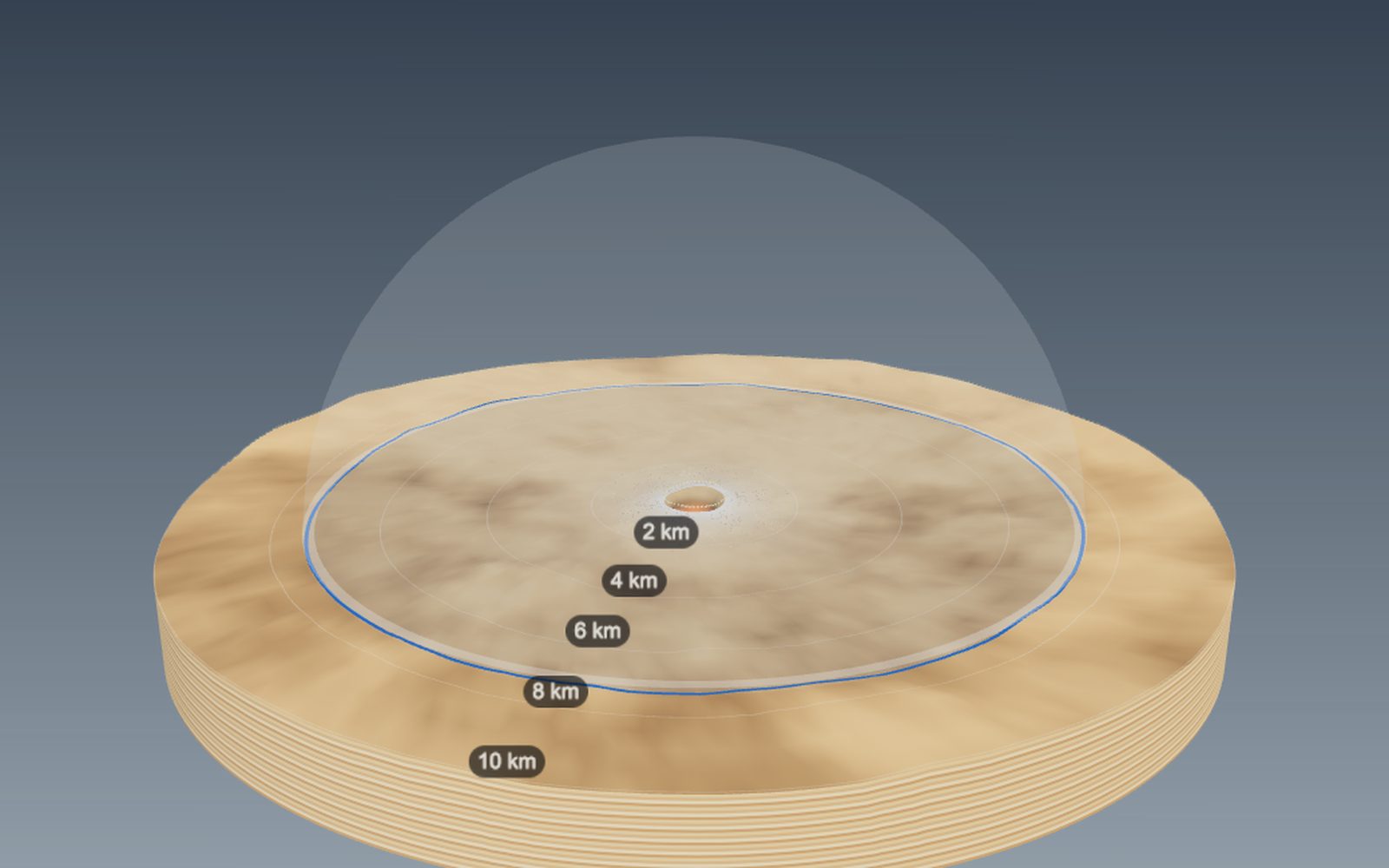
How big a crater would an asteroid make, and how craters form
The 1.2 km wide Meteor Crater in Arizona was dug by an iron asteroid only a few tens of metres across.
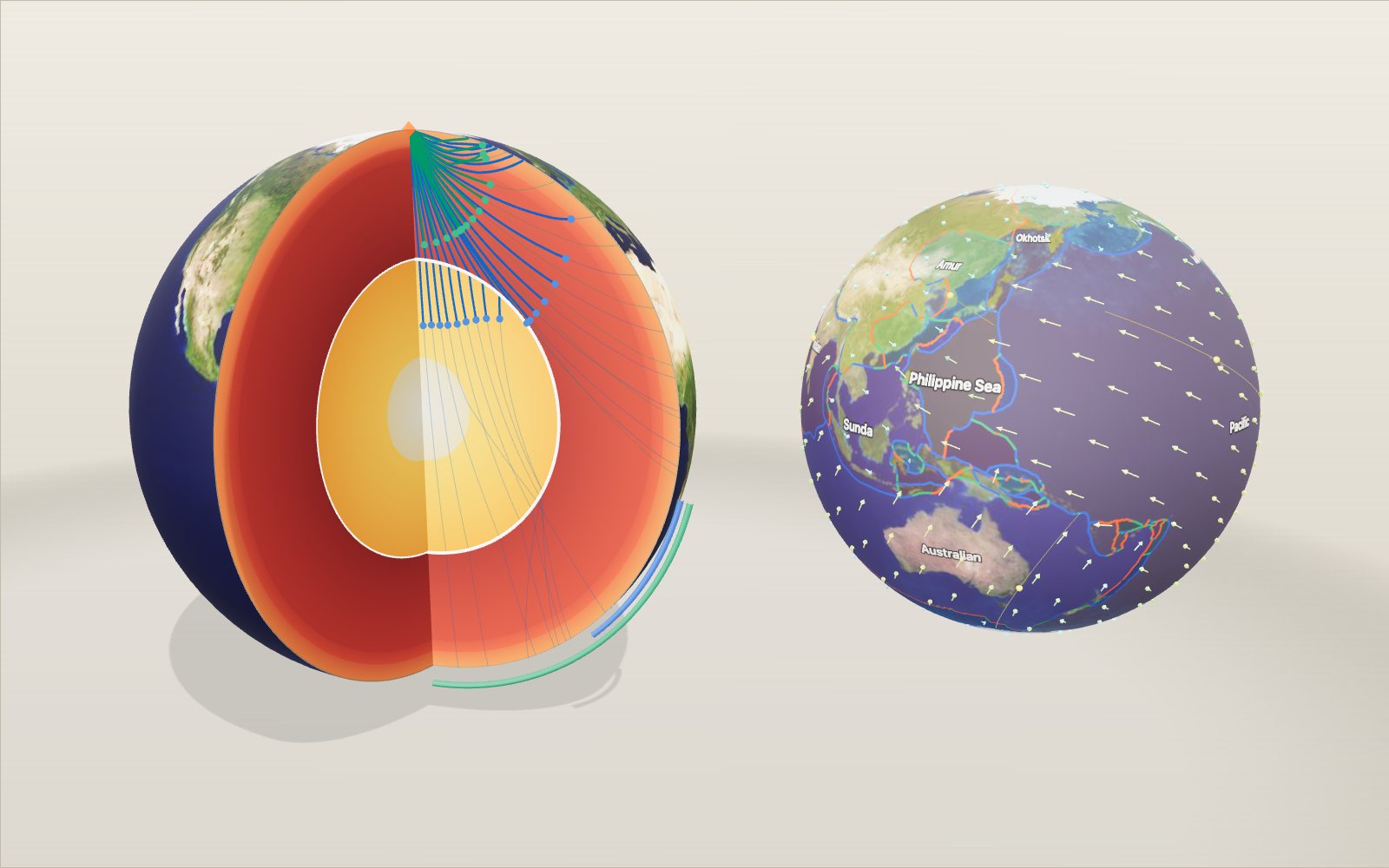
Layers of the Earth: depth and density, interactive model
Nobody has drilled deeper than 12.3 km, yet we know the pressure at the centre to within a few per cent, because earthquakes shine through the planet.
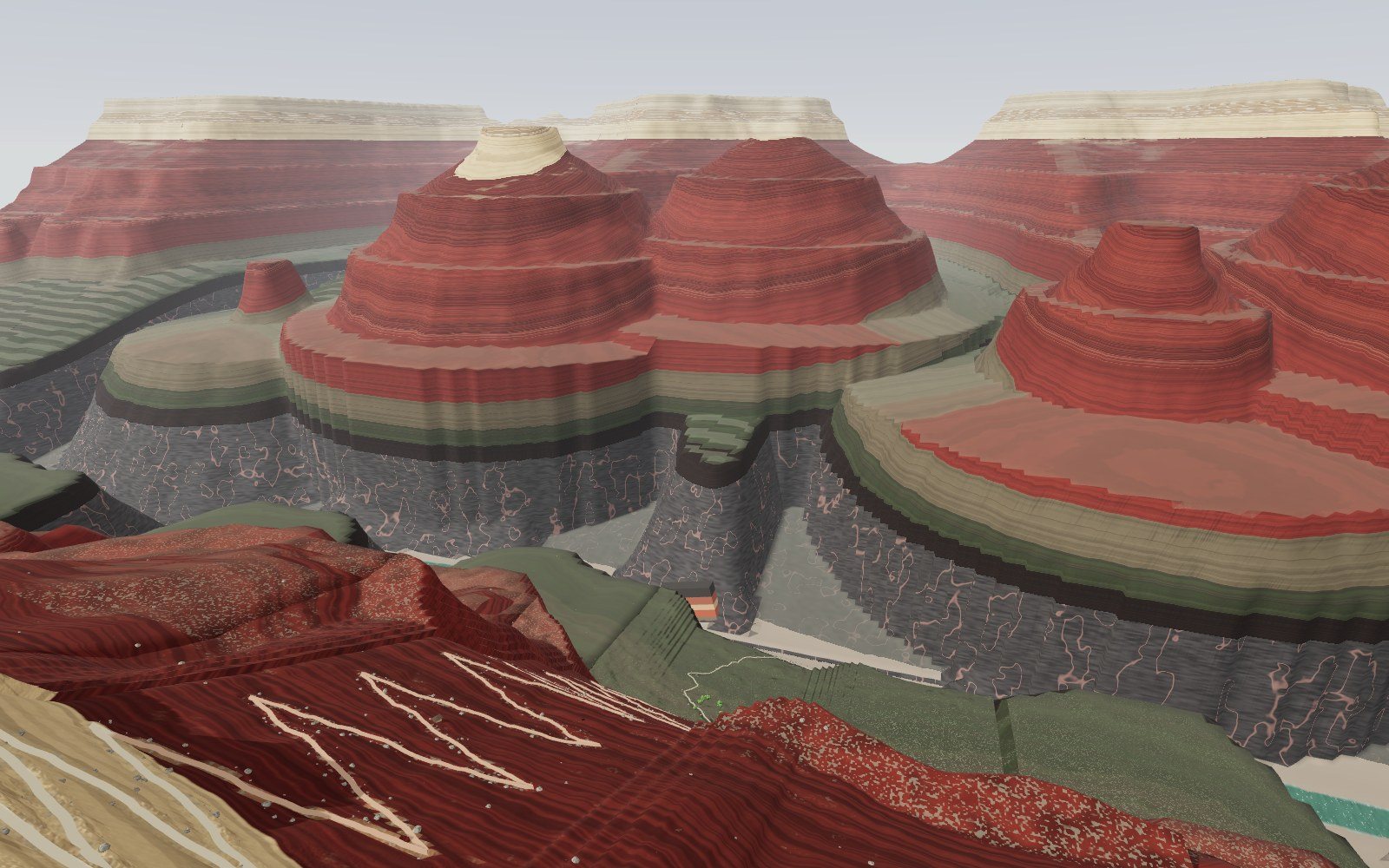
Walk down the Grand Canyon rock layers
Walk 1,360 m down the Bright Angel Trail through 13 rock layers, from a 270-million-year-old sea floor on the rim to 1.75-billion-year-old schist by the river.
Why salt forms cubes: crystal structure and unit cells
A grain of table salt is a stack of cubes 0.564 nm on a side, with sodium and chlorine alternating along every edge.
Where volcanoes and earthquakes happen
For each second between the P wave and the S wave, the earthquake is roughly 8 km farther from the seismometer.
Origami: 20 models to fold step by step and unfold
A crane uses about 30 folds, a cup six; every flat-folded point you make has mountains and valleys that differ by exactly two.